In this Excel tutorial, you will see and learn, why it is a good idea to use the Match function in Vlookup formula.
By using Vlookup and Match formula together you can make Vlookup column number input dynamic.
Using the Match formula in Vlookup has below advantages
- Build Vlookup formula in one cell and copy to other cells without manually editing column number in each cell
- Get information of any field ad-hoc basis
- Saves formula writing time
Use Vlookup and Index formula to save formula writing time
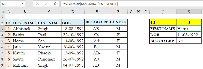
In the below image cell K3 formula is
=VLOOKUP($K$2,$A$2:$F$9,2,FALSE)
Here, column number input is static.
For DOB and Blood Grp output you have to copy the formula then manually change the column number input to 4 and 5 respectively.
In this case, only 3 fields (columns) information you have to fetch.
Imagine if you have to get information of 10 or more fields (column) then manually editing column number in the Vlookup formula for each field is going to be laborious, time-consuming, and prone to error.

To dynamically set lookup column number in Vlookup, Match function can be used.
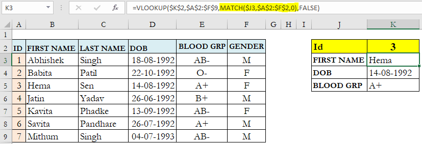
Updated cell K3 formula
=VLOOKUP($K$2,$A$2:$F$9,MATCH($J3,$A$2:$F$2,0),FALSE)
In the above formula, you can see Match function is used at the place of the lookup column value.
Match function evaluation in cell K3
MATCH($J3,$A$2:$F$2,0) > MATCH(“FIRST NAME”,$A$2:$F$2,0) > 2
In range $A$2:$F$2, “FIRST NAME” is in second cell hence output is 2.
Note:- Take care of selecting 2nd input (range) in Match function, so that Match function output, mimics the manual input of column number.

For First Name Match function will output 2 , for DOB 4 and for Blood Grp 5.
Note:- One should always use 0 in third input of Match function for finding the exact position of matched valued in a range.
Also, the Heading value and lookup value of the Match function must be the same. Notice cell J3 and B2 values are the same.

You have to write this Vlookup and Match combination formula in cell K3 and just copy-paste the formula in lower cells (K4 to K5), no need to manually change the lookup column number for each information.
You can clearly see this will save formula writing time if you have to lookup many fields from a table.
The match function will take care of dynamically changing the lookup column number.
Get information of any field ad-hoc basis
Suppose you have a table having more than 10 or more columns (fields).
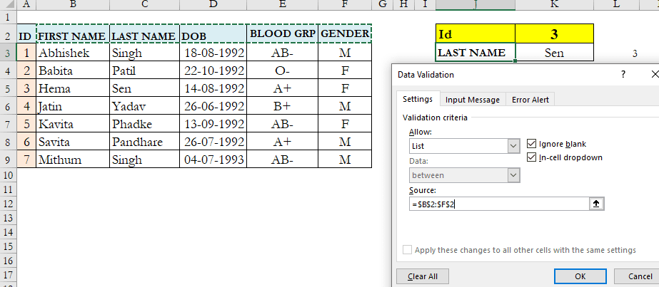
You want to dynamically get the information of the column (field) selected from the drop-down list.
In the below image example only one drop-down list is shown but you can create many as per your requirement using the same method.

Follow the below steps to create this type of utility in Excel
- Select the cell (Cell J3) in which you want to have a drop-down list the press ALT D L keys in series to bring Data Validation pane.
Alternatively, you can go to the Data tab then select the Data validation option.
-
- In Allow select List. In Source select the table heading range and press OK button.

- In cell, K3 write Vlookup and Match combination formula
=VLOOKUP($K$2,$A$2:$F$9,MATCH($J3,$A$2:$F$2,0),FALSE)
Now you are done.
When a new column name from the drop-down list is selected then its respective value gets auto-updated.
Here Match function dynamically determines (auto-updates) the column number in the Vlookup formula.
Suggested Readings
Return multiple Vlookup values in one cell (Text join if) 3 ways
Two way lookup in Excel | Excel two way lookup Index Match
Reverse Vlookup In Excel (Vlookup Right to Left)
Vlookup to return all matched values in Excel (return multiple matches) using 3 ways