December 2020 – LearnYouAndMe

Typically, you Vlookup data from a single Vlookup table or table array but sometimes, you may find a situation where you have to lookup tables, present across different worksheets or sheets of a workbook.

In this article, I will show you 4 ways to Vlookup (lookup) across multiple sheets.

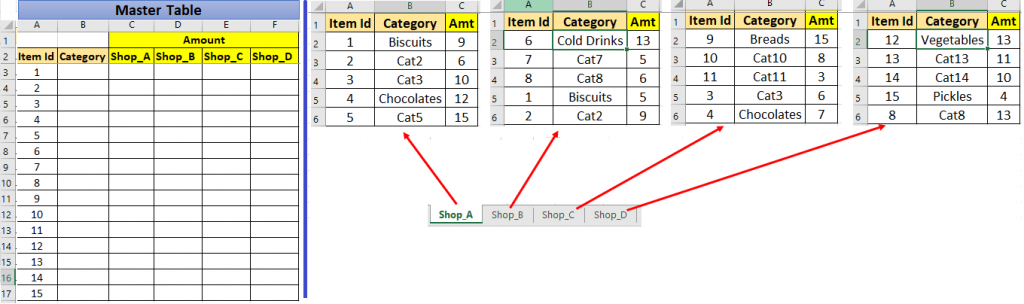
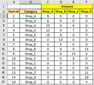
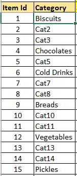
In the below image you can see in the left-most table (Master Table) we have to bring amount and Category values using Vlookup. On the right side, you can see four small tables present in different sheets.

Here our task is to get Category and Amount values from these four tables using Vlookup.

Using combination of Vlookup and Indirect (non array formula)

First, I will bring Amount values.

Here idea is to dynamically change Vlookup table reference using Indirect function for each amount column in Master Table.

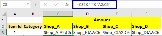
In cell C3 write below formula =C$2 & “!” & “A2:C6”,

This will give text range reference of lookup table range for each shop.

Note:- As you can see in range C2 to F2 heading are exactly equal to sheet names in which lookup tables are present, this you should take care of.

Now if sheet name contains space like Shop A instead of Shop_A then formula becomes =”‘” & C$2 & “‘!” & “A2:C6” which will output ‘Shop A’!A2:C6.

In my personal opinion it is better to have sheet names without space for making formula less complex.

Also note that lookup tables in four sheets starts with same cell which is Cell A1, also heading order is also same in these lookup tables.

Now I will wrap the above formula in Indirect function to make it a range reference.

Cell C3 formula =INDIRECT(C$2&”!”&”A2:C6″,TRUE)

Now after applying Indirect formula, our text range reference got converted in actual range which is our lookup table or table array.

=INDIRECT(C$2&”!”&”A2:C6″,TRUE) is equivalent to =Shop_A!A2:C6 when you manually give reference.

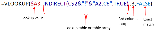
Cell C2 formula =VLOOKUP($A3,INDIRECT(C$2&”!”&”A2:C6″,TRUE),3,FALSE)

Know about Indirect function

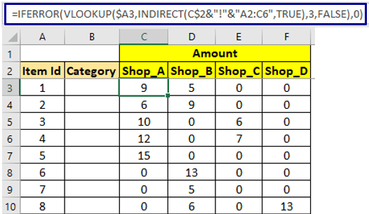
To remove error #N/A from Vlookup output just wrap it in IFERROR function.

Cell C3 formula =IFERROR(VLOOKUP($A3,INDIRECT(C$2&”!”&”A2:C6″,TRUE),3,FALSE),0)

Now you have to just copy paste this in all the amount cells.

Note that you have to build above formula in only one cell then just copy paste in other cells.

Using array formula

After amount Vlookup across multiple sheets I will do category Vlookup across multiple sheets.

For category Vlookup if I will apply same above formulas then I will not look good and will need another 4 more columns and this will lead to increase in file size.

Cell B3 formula =VLOOKUP(A3,INDIRECT(INDEX($C$2:$F$2,1,MATCH(TRUE,

COUNTIF(INDIRECT($C$2:$F$2&”!A2:A6″),A3)>0,0))&”!A2:C6″),2,FALSE)

This formula is array so you have to press CTRL+SHIFT+ENTER instead of ENTER after writing formula.

Working of Vlookup across multiple sheets array formula

Let’s understand above formula working.

=VLOOKUP(A3, someMagicalFormula , 2 , FALSE)

=VLOOKUP(A3, INDIRECT(INDEX($C$2:$F$2,1,MATCH(TRUE,COUNTIF(INDIRECT($C$2:$F$2&”!A2:A6″),A3)>0,0))& “!A2:C6”) , 2 , FALSE)

If you carefully look at the above Vlookup formula then the yellow part is somehow outputting a dynamic Vlookup table range or table array.

INDIRECT(INDEX($C$2:$F$2,1,MATCH(TRUE,COUNTIF(INDIRECT($C$2:$F$2&”!A2:A6″),A3)>0,0))& “!A2:C6”)

Now in the above Indirect formula section red part must be giving the sheet name which is then concatenating with a range which is the blue part.

So for item id. 1, it must look like INDIRECT(Shop_A &“!A2:C6”) which becomes INDIRECT(Shop_A“!A2:C6”) .

And for item id. 6, it must look like INDIRECT(Shop_B &“!A2:C6”) which becomes INDIRECT(Shop_B“!A2:C6”) and so on. This indirect function eventually represents a range.

INDEX($C$2:$F$2,1,MATCH(TRUE,COUNTIF (INDIRECT($C$2:$F$2&”!A2:A6″) ,A3)>0,0))

Yellow sub section of above formula will give array of Item Id range address of four Vlookup tables.

Select yellow section and press F9 function key you will see something like below

INDIRECT({“Shop_A!A2:A6″,”Shop_B!A2:A6″,”Shop_C!A2:A6″,”Shop_D!A2:A6”}) , now these array values will converted into a range because of Indirect function.

COUNTIF (INDIRECT({“Shop_A!A2:A6″,”Shop_B!A2:A6″,”Shop_C!A2:A6″,”Shop_D!A2:A6”}) ,A3)

here cell A3 value is 1, so this section will perform Countif operation for each range of an array.

If you select this COUNTIF(INDIRECT($C$2:$F$2&”!A2:A6″),A3) section and hit F9 then this will be shown {1,1,0,0}

COUNTIF(INDIRECT($C$2:$F$2&”!A2:A6″),A3)>0 section is there for managing more than 1 count ({1,1,0,0}>0)

Above is evaluated to {TRUE,TRUE,FALSE,FALSE} true means Item id. 1 is present in 1^st and 2^nd sheet.

MATCH(TRUE,COUNTIF(INDIRECT($C$2:$F$2&”!A2:A6″),A3)>0,0) will give 1^st matched value of True.

MATCH(TRUE, {TRUE,TRUE,FALSE,FALSE},0) will output 1.

If you see the above image you can correlate output produced in Category column and values in range (C2 to F2).

1 means 1^st value of range C2 to F2, 2 means 2nd value of range C2 to F2

=INDEX($C$2:$F$2,1,MATCH(TRUE,COUNTIF(INDIRECT($C$2:$F$2&”!A2:A6″),A3)>0,0))

will give sheet name in which Item Id is first found.

Now you are almost done just use another Indirect function to refer Vlookup table range dynamically.

INDIRECT(INDEX($C$2:$F$2,1,MATCH(TRUE,COUNTIF(INDIRECT($C$2:$F$2&”!A2:A6″),A3)>0,0))& “!A2:C6”) this will give

INDIRECT(Shop_A&“!A2:C6”) which is eventually a range of Shop_A sheet.

Now apply Vlookup formula

=VLOOKUP(A3, someMagicalFormula , 2 , FALSE)

=VLOOKUP(A3, INDIRECT(Shop_A&“!A2:C6”) , 2 , FALSE)

=VLOOKUP(A3, Shop_A“!A2:C6” , 2 , FALSE) which will output Biscuits.

Vlookup across multiple sheets using helper UDF (User Defined Function)

So, as you can see whole complexity is there for outputting Sheet name in which Item id. is first found.

Can we simplify this, yes using VBA UDF (User Defined Funtion).

You may say UDFs are slow but I have optimized this UDF and tested it over 10 thousand (10K) cells, all 10K cells got calculated in less than 10 seconds which is pretty much fast.

Not able to believe just do below things from your side.

Press ALT + F11 to open VBA IDE and create one standard module. Click on Insert tab then click on Module.

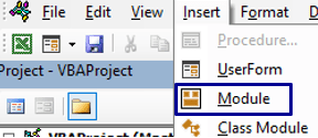
Double click on newly created module and copy paste below code in that module.

Note:- VBA UDF must be written in Standard module otherwise you will be not able to use UDF in Excel cell or Excel user interface.

Option Explicit
Option Compare Text
Function foundInSheetNm _
(shtNmRng As Range, rngRef As String, findVal As Range) As String
  Dim cel As Range, shtNm As String, mtchIdx As Long
  
  For Each cel In shtNmRng
     On Error Resume Next
      mtchIdx = Application.WorksheetFunction. _
      Match(findVal.Value, Sheets(cel.Value).Range(rngRef), 0)
     If mtchIdx > 0 Then
        shtNm = cel.Value
        Exit For
     End If
  Next cel
  
  If shtNm = "" Then Exit Function
  If InStr(shtNm, " ") = 0 Then
    foundInSheetNm = shtNm & "!"
  Else
    foundInSheetNm = "'" & shtNm & "'" & "!"
  End If
End Function

Don’t forget to save as you Excel file either in .XLSB (binary) or .XLSM (macro) format else you UDF will not be saved for future use.

As you can see function or UDF name is foundInSheetNm which gives sheet name in which particular value is found in a given range.

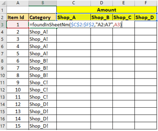
Cell B3 formula =foundInSheetNm($C$2:$F$2,”A2:A7″,A3)

In the above formula 1^st input is range in which sheets names are present

2^nd input is range A2:A7 (Item id range) in which we have to find a value

3^rd input is which value (A3 which is Item id.) we have to find in respective sheets and their respective range.

In the below image this foundInSheetNm UDF function is outputting Sheets name in which Item Id is found this means core of issue is solved.

Now you just have to use Indirect function to make dynamically refer Vlookup table or table array of a given sheet

Cell B3 formula =INDIRECT(foundInSheetNm($C$2:$F$2,”A2:A7″,A3) & “A2:C7”)

After this just use above formula as table_array or Vlookup table of Vlookup formula.

Cell B3 formula =VLOOKUP(A3, INDIRECT(foundInSheetNm($C$2:$F$2,”A2:A7″,A3)&”A2:C7″) , 2,FALSE)

Above formula takes less than 10 seconds for 10K cells to give output.

Just copy paste the above formula in the below cells it will give output as per the below image.

Click to download the workbook for this UDF

Note:-UDFs will only work in workbooks in which UDF code is written and not available to another workbook.

Make UDF (User Defined Function) available in all the open workbooks

How to make UDF (User Defined Function) in Excel

Note:- All UDF calculation time testing is done by opening only one workbook so as to maximize speed.

Calculation time may increase when multiple workbooks are open and other resource intensive applications are open. My Hardware property 4GB RAM, i5 2.60 GHz processor.

Using super advance UDF (10 thousand cells less than 1.10 min ( 70 seconds))

This UDF (User Defined Function) for multiple sheet Vlookup is super advance and flexible.

In the above examples lookup tables or table array have same starting cell of table which is Cell A1, also column’s orders are same.

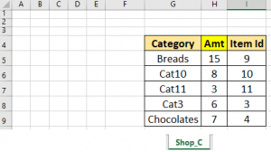
Now consider scenario where in each sheet lookup table starting cell is different and also column order is different like the below image.

In Shop_C sheet I have changed the column order also starting cell of table which is cell G4.

This multiple sheet Vlookup UDF is designed to handle this type of scenario or irregularity.

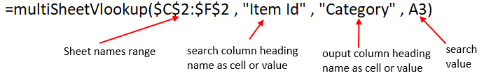
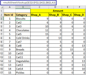
Cell B3 formula =multiSheetVlookup($C$2:$F$2,$A$2,$B$2,A3)

multiSheetVlookup VBA UDF function inputs

1^st input is range having sheets names

2^nd input is lookup column heading as range or heading name( column in which Vlookup value will be found)

3^rd input is output column heading as range or heading name (column whose cell value you want to output)

4^th is which value you want to search in lookup column of lookup table

Cell B3 formula can also be written as =multiSheetVlookup($C$2:$F$2,”Item Id”,”Category”,A3)

Cell C3 formula =IFERROR(multiSheetVlookup(C$2,$A$2,”amt”,$A3),0)

Note:- Since this VBA UDF works on heading names of lookup tables hence make sure all table have same heading spelling.

Column order can be different, it does not matter to this VBA UDF.

Paste below VBA UDF code in standard module to use it in a cell

Option Explicit
Option Compare Text

Function multiSheetVlookup _
(shtNmRng As Range, headVal As String, outPutHd As String, findVal As Range) As Variant
 Dim shtNmAr As Variant, nm As Variant, mtchIdx As Long, fndVl As Variant
 Dim sht As Worksheet, findInRng As Range, outRng As Range
  shtNmAr = shtNmRng.Value2
  fndVl = findVal.Value
  
  If shtNmRng.Cells.Count = 1 Then
    nm = shtNmAr
    GoTo lp:
 End If
     
  For Each nm In shtNmAr
lp:
  On Error Resume Next
  
     Set sht = Worksheets(nm)
    If sht Is Nothing Then GoTo jmp
    
    Set findInRng = sht.UsedRange _
    .Find(what:=headVal, LookIn:=xlValues, lookat:=xlWhole, MatchCase:=False)
    If findInRng Is Nothing Then GoTo jmp
    Set findInRng = sht.Range(findInRng, findInRng.End(xlDown))
        
     Set outRng = sht.UsedRange _
    .Find(what:=outPutHd, LookIn:=xlValues, lookat:=xlWhole, MatchCase:=False)
    If outRng Is Nothing Then GoTo jmp
    Set outRng = outRng.Resize(findInRng.Rows.Count, 1)
      
     mtchIdx = Application.WorksheetFunction.Match(fndVl, findInRng, 0)
     If mtchIdx = 0 Then GoTo jmp
     multiSheetVlookup = Application.WorksheetFunction.Index(outRng, mtchIdx, 1)
     Exit For
jmp:
  Next nm
  
  If multiSheetVlookup = 0 Then multiSheetVlookup = CVErr(xlErrNA)
End Function

Advantages of multiSheetVlookup VBA UDF function

Can do left right and right to left Vlookup (not to worry about column’s order) .
Can be used as alternate of Vlookup from different sheets of same workbook.
Can do Vlookup even when table range address of each lookup table is different in each sheet.
Fairly fast.

Click to download the workbook for this UDF