Microsoft Excel is one of the most widely used software for data crunching and reporting. In Excel you can do a specific task in more than one way.
But one way is more efficient or productive than another method for the same task.
Though list can be many for increasing Excel productivity but here I will share 12 ways to boost your Excel productivity.
Wonder of Subtotal Function in Excel
I have seen Excel users selecting filtered value range for getting Sum or total at status bar.
Instead of selecting filtered range each time then seeing Sum at status bar, use Subtotal function.
Subtotal function dynamically performs calculations only on visible cell values in filtered range. Using Subtotal you can do Sum, Count, Average, Product and so on.
Syntax :- =SUBTOTAL(function_number,range)
Function number represents the type of calculation you want to perform on visible cells or filtered range like use 9 form Sum and 1 for Average.
Watch video version
Very useful Excel Subtotal formula
Shortcut key for Subtotal formula (trick)

Use Quick Access Toolbar
Excel shortcut keys are good for fast pace work in Excel.
But, not all Excel features or tools have shortcut key or even if they have they are longer, more than 2 or 3 keys combination.
Quick Access Toolbar helps in
- Making longer shortcut key even shorter
- Makes any feature one mouse click way
Suppose in Excel you have to frequently use Wrap text , to do this you click on the Home tab then click on wrap text (2 mouse clicks) or press ALT H W keys (3 keys) in series (keyboard accelerator).
Using quick access toolbar you can make Wrap text one mouse click away and shorten your shortcut key to 2 keys.
To add Wrap text or any feature in Quick Access Toolbar bring cursor on that feature, here feature is Wrap text then right mouse click then click on Add to Quick Access Toolbar.
Now wrap text got added in Quick Access Toolbar (QAT) you can just directly click on that to use it.
Or you can press ALT key then see at which number that feature is there in QAT then leave ALT key and press that number to use that feature.
Note:- ALT Number key series will vary from user to user.

To remove a feature or tool from Quick Access Toolbar just place mouse cursor on that quick access toolbar then right mouse click then click on Remove from Quick Access Toolbar.

Use Excel Named range
By using Named range you can give meaning full name to specific range. Named range also called address naming.
Example:- In a sheet from A1 to A5 category values are present but using named range you can name or represent A1:A5 as Category.
Effects of named range
- More readable formulas
- Quick navigation to a specific range
- Objectifying range or organizing data more meaningful way
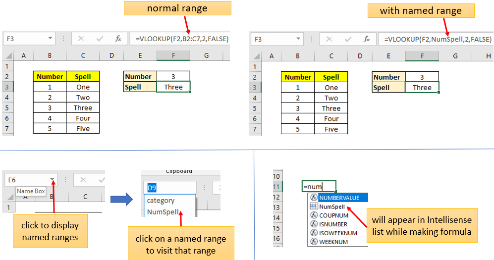
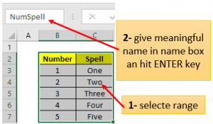
To create Named range select a range then in Name Box write meaningful name then hit ENTER key.
Note:- Naming must be without space and should not start with numbers and special characters. Also naming should not coincide with cell address like AA1, Z1 etc.
Quickly generate series in Excel
Many times in Excel you are required to generate number series like 1 to 10 or even number series or list of Month names or list of Weekday names.
Instead of typing list values manually you can use autofill series or auto fill list feature of Excel.
Go generate number series, write first 2 numbers then select cells, Fill Handle or drag tool tip will appear, mouse click on this drag tool tip (+ sign) and drag mouse keeping mouse button pressed.

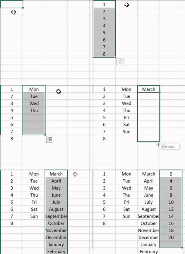
Note:- If Fill Handle not visible then click on File tab then click on Options then select Advance, in Editing section tick on Enable Fill Handle and Cell Drag and Drop option then click on Ok.

In addition to inbuilt pre-defined lists like Month name, Weekday name you can custom build your own list.
Click this link to watch how to build or add custom list in Excel.
Quickly copy paste without using CTRL+C and CTRl+V
Many times you can copy paste formula or values without using CTRL+C and CTRL+V.
Use CTRL+R to quickly copy paste value or formula in just Right cell from left cell.

Use CTRL+D to quickly copy paste value or formula in just lower (Down) cell from upper cell.

Quickly fill blank cells with upper value |Fill down blank cells
Sometimes you may required to fill down upper value in lower blank cells like the below image.
If you want to apply Pivot Table or apply formula like Sumif,Countif Etc. or want to do some kind of data analysis then your table must look like the right one without any blank cells.

Here are steps to fill down blank cells in Excel
- Select you table range
- Keeping selection intact, press F5 function key. Click on Special (at bottom).
- In Go To Special pane tick on Blanks then click on Ok. This will select all the blank cells.
- Keeping blank cells selection intact, in active cell write formula =upperCellAddress (Example = C3 if C2 is active cell). Then press CTRL+ENTER.
- Now all blank cells will get filled with upper cell values. Now copy your table range then paste special as value to remove formulas and keeping only values.

Watch video version
Quickly fill down blank cells with upper cell value in Excel
Quickly select and color all formula cells
You may required to select and color only formula cells so that you can differentiate between entry cell and formula cell.
You may say what is the big deal just manually select formula cells then color it.
In real scenario one a sheet can have many formula cells scattered across different cells and in that case it is time consuming to see and select formula cells manually.
Here are the steps for quickly selecting all formula cells in a worksheet then coloring it.
- Select all the cells of a sheet by mouse clicking on select all cells sign. Select all cells sign is present at upper left corner of row and column heading.
- Keeping cells selected, press F5 function key. Then click on Special to bring Go To pane.
- In Go To pane tick Formulas then click on Ok. This will select all formula cells automatically.
- After selecting formula cells you can color those cells. By going in Home tab and using Fill Color option.
You can go one step further by protecting formula cells so that user is not able to delete or modify formulas accidently.

Quickly adjust column width in Excel
To quickly adjust column width in Excel just select cell or range then press ALT H O I keys in series (do not keep hold the previous key).
If you find ALT H O i too long then add Autofit Column Width tool in Quick Access Toolbar. Autofit Column Width present in Home tab in Format option drop down.
Alternatively, hover cursor between column head and mouse double click. Refer below image for more clarity.

Reduce Excel file Size to save disc space and upload quickly
If you have a heavy Excel file and want to reduce it then save as your Excel file in Binary format (.xlsb).
Press F12 function key then in Save as Type dropdown select Excel Binary Workbook to save Excel file in Binary format.
Excel Binary format file reduces file size by 20 to 30 percent (effect more visible heavy files).
Binary Excel file have all the features of default Excel file format (.xlsx).
By reducing Excel file you save your disc space also online upload time is reduced.
Watch video version
How to reduce large excel file size in few seconds using excel binary format?
Use Excel Table (underutilized but very useful)
Excel table is one of my favorite Excel feature. In VBA, Excel is known as List Object.
To make normal table a official Excel table select table range then press CTRL+T , make sure to tick on My table has headers then click on Ok.
Alternatively,select table range then go to Insert tab then click on Table option.
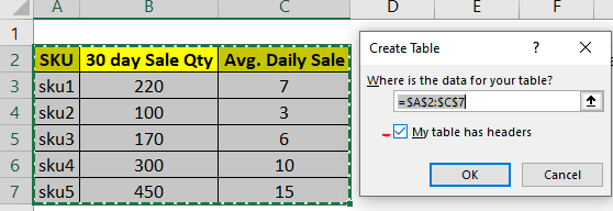
Advantages of Excel Table
- Formula will get autofilled and auto extended when new row or record is added.
- Formula referring to table cell is more readable.
- Named range of table gets auto created thus helping in quick navigation.
Watch the below video to know one of the usage of Excel Table.
Record Macro for repetitive task (use VBA)
Excel Macros are great for automating any repetitive task.
While recording macro, whatever you do in Excel is just get converted into code behind the scene. You can see macro code in VBA IDE by pressing ALT+F11.
By recording macro you can make any task button click away.
You can also assign shortcut key to that macro. After pressing shorcut key macro will run and you taks will get done.
To record a macro follow the below steps
- Make sure the developer tab is visible, if not then click on File tab then Options. Click on Customize Ribbon. At right side find Developer option and tick it then click on Ok.
- In Developer tab click on Record Macro to start recording macro.
- Perform specific actions which you want to automate then click on Stop Recording.

Watch the below videos related to macro recoding in Excel.
Learn to record your first Excel macro
How to give or change macro/VBA shortcut key
Various ways to run VBA or macro
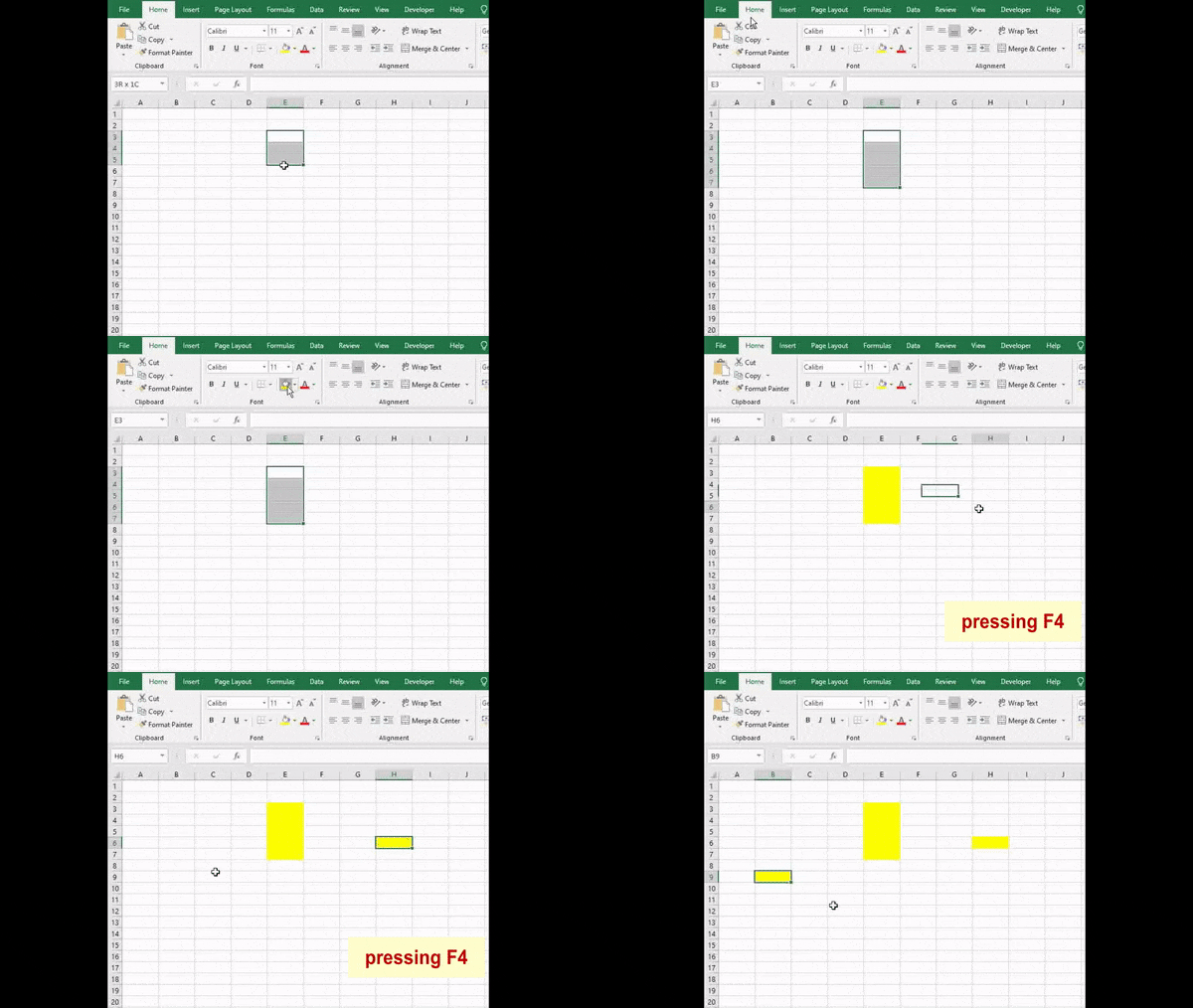
Use F4 function key
F4 function key is great for repeating recent action done in Excel.
Suppose you color some cell or range by going in Home tab using mouse.
If you want to repeat that action (coloring cell with same color) then you can press F4 function instead of going in Home tab.
