In this article, I will show you how to do two way lookup in Excel.
I will use two ways for this, first one is using Vlookup and Match function and the second is using Index Match function.
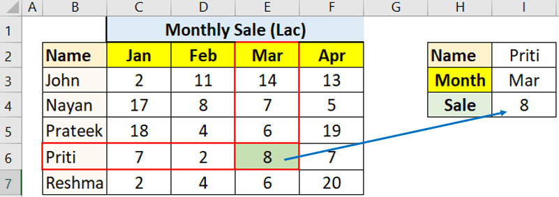
In two way lookup you have to lookup, lookup value also its respective output column dynamically. Thus it is two dimension lookup.
See the below image to get clarity about tow way lookup in Excel.
On changing Name and Month sale must be updated automatically.

Two way Lookup using Vlookup and Match (exact type)
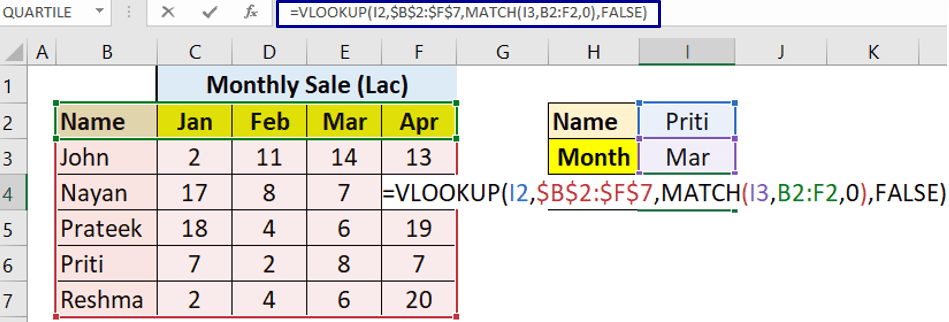
In this method I will use combination of Vlookup and Match function.
If you carefully look at the above image it can be done with sime exact Vlookup function with small twist.
And that small twist is Match function for auto calculating column index number of Vlookup formula.
Priti sale for March month simple Vlookup formula is below
=VLOOKUP(I2,$B$2:$F$7,4,FALSE)
In the above Vlookup formula I want 3rd input to get dynamically calculated using Match function as Month changes.
After inserting match function Vlookup formula will look like below
=VLOOKUP(I2,$B$2:$F$7,MATCH(I3,B2:F2,0),FALSE)

Two way lookup with Index Match (exact type)
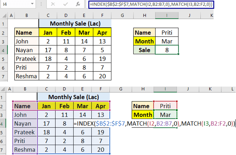
Using Index Match the formula will be
=INDEX($B$2:$F$7,MATCH(I2,B2:B7,0),MATCH(I3,B2:F2,0))

Formula Working
First look at basic syntax of Index function
Index(range,[row number],[column number])
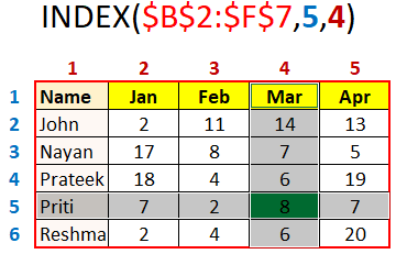
So , in case of Priti and March month formula will be
=INDEX($B$2:$F$7,5,4)
What above formula means is that in range $B$2:$F$7 output a cell reference which is intersection of 5th row and 4th column in $B$2:$F$7 range.

In the above Index formula I want [row number] and [column number] to get calculated automatically when name and month changes.
To make it happen MATCH(I2,B2:B7,0) is used to auto calculate [row number]
and MATCH(I3,B2:F2,0) is used to auto calculate [column number].
So final complex formula will be like the below
=INDEX($B$2:$F$7,MATCH(I2,B2:B7,0),MATCH(I3,B2:F2,0))