Sometimes you may want to perform Excel calculations like Sum,Count,Max,Min based either cell color or font color. In this article I will show you various ways to Sum or do other calculations based on color in Excel.
I have included without VBA method and using VBA UDF for doing Sum based on color.
This article also shows to Sum conditional formatted colored cells along with manually colored cells.
Sum colored cells in Excel without VBA using filter and Subtotal
Using this approach you perform any calculations based like Sum,Count,Max,Average ETC. offered by Subtotal function.
One drawback of this approach is that you can do calculations based on one color at a time. This will work for both conditional formatted color and manually colored cell.
In the below image you can see a table having Sales (Lac) column and cells are colored higher value greener side and low value red side.
Here I want Sum of dark green cell values.
For this first write Subtotal formula for Sum in Cell C1 like below ( you can also write this formula in any other cell also).
=SUBTOTAL(9,$C$2:$C$16)
2nd select heading row and press CTRL+SHIFT+L to apply filter.
In sales column drop down button select Filter By Color then in Filter by Cell Color, select color which you want to filter for me it is dark green.
Note:- You can also use Filter by Font Color, since all font have default color in Sales column hence Filter By Color only showing Filter By Cell Color.
Subtotal function dynamically does calculations on visible cells only.
In the right image you can see cell C1 output is 365 which is sum of all the values.
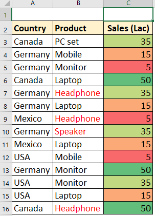

After filtering by dark green color you can see only green color cells are visible and whose sum is ouputted in cell C1 having subtotal function for sum.
For getting sum of other color just remove filter then select that color in Filter by Cell color option.
Yon can perform all the calculations which Subtotal offers (22 functions) .
For Max use =SUBTOTAL(4,C2:C16), for Count use =SUBTOTAL(2,C2:C16)
For product use =SUBTOTAL(6,C2:C16)

Sum colored cells and colored font using helper VBA UDF and helper column
This method is very flexible , using helper column you can perform all the available functions of Excel like sum, sumif,count,countif Etc based on cell color.
Note:- This method is only for manually colored cell background or font color not conditionally formatted color.
For using this method you have to create one UDF function named getColorNo.
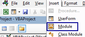
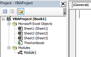
To create below UDF press ALT+F11 to open VBA IDE. In VBA IDE go to Insert tab and click on Module to create new standard module. Now copy paste below code section in that module.
Make sure to save as your workbook either in .xlsb (binary) or .xlsm (macro) format.
Function getColorNo(rng As Range, Optional isFontClr As Boolean = False) As Long
  Application.Volatile
  If isFontClr Then
     getColorNo = rng.Font.Color
  Else
     getColorNo = rng.Interior.Color
  End If
End Function
After copy pasting UDF in Module you are ready to use getColorNo UDF function in Excel cell.
1st create two helper colmuns one for cell color and one for font color like the below image. Now apply getColorNo UDF function in these two columns. cell D3 formula =getColorNo(C3)
cell E3 formula =getColorNo(C3,TRUE)
1st input is the cell whose background color or font color value you want to get. Write only 1st input if you want to get cell background color value.
2nd input is optional and accepts boolean values (True/False). To get font color value input True as 2nd input.
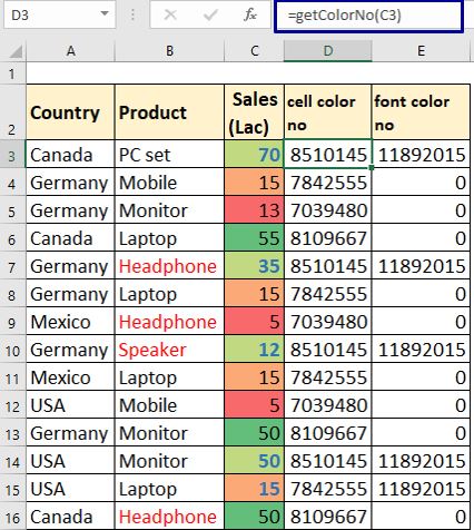
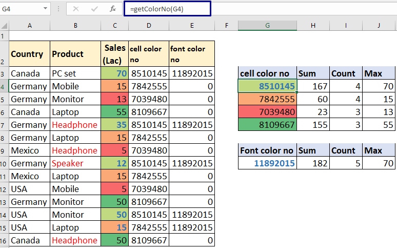
After getting respective color values using getColorNo UDF in helper columns you are ready to rock and you can apply any Excel function as per your need.
Cell G4 formula =getColorNo(G4), cell H4 formula =SUMIF($D$3:$D$16,G4,$C$3:$C$16), cell I4 formula =COUNTIF($D$3:$D$16,G4), cell J4 formula =MAXIFS($C$3:$C$16,$D$3:$D$16,G4)
cell G10 formula =getColorNo(G10,TRUE) , cell H10 formula =SUMIF($E$3:$E$16,G10,$C$3:$C$16), cell I10 formula =COUNTIF($E$3:$E$16,G10), cell J10 formula =MAXIFS($C$3:$C$16,$E$3:$E$16,G10)
Note:- If you change color of any cell then formula output will not get auto-updated. To get new updated output value just double mouse click on formula cell (or select formula cell then press F2) then press Enter key or enter new value in any blank cell.
Direct VBA UDF to sum colored cells and colored font
To create below coloredValAr UDF press ALT+F11 to open VBA IDE. In VBA IDE go to Insert tab and click on Module to create new standard module. Now copy paste below code section in that module.
Make sure to save as your workbook either in .xlsb (binary) or .xlsm (macro) format.
Function coloredValAr(rng As Range, equalToClrCel As Range, _
Optional isFontClr As Boolean = False) As Variant()
    Application.Volatile
  Dim cel As Range, nwAr() As Variant, i As Long, eclrVal As Long
  i = 0
   If isFontClr Then
     eclrVal = equalToClrCel.Font.Color
   Else
     eclrVal = equalToClrCel.Interior.Color
   End If
   If isFontClr Then
     For Each cel In rng
       If cel.Font.Color = eclrVal Then
         ReDim Preserve nwAr(0 To i)
         nwAr(i) = cel.Value
         i = i + 1
       End If
     Next cel
  Else
      For Each cel In rng
       If cel.Interior.Color = eclrVal Then
         ReDim Preserve nwAr(0 To i)
         nwAr(i) = cel.Value
         i = i + 1
       End If
     Next cel
  End If
    coloredValAr = nwAr
End Function
Above UDF is only for manually colored cells or font not conditionally formatted cells.
After copy pasting UDF in Module you are ready to use coloredValAr UDF function in Excel cell.
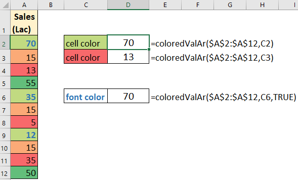
First understand what coloredValAr UDF does. This UDF basically outputs array of values which is matched with a give cell color or font color.
Cell D2 formula =coloredValAr($A$2:$A$12,C2)
Cell D6 formula =coloredValAr($A$2:$A$12,C6,TRUE)
1st input is range which contains colored cells or fonts, 2nd input is cell which represents equal to which color or font color, 3rd input is whether font color or cell background color.
If based on font color then input True else fill only first two inputs.
Double mouse click D2 cell to display formula (or press F2 ) then press F9 to see evaluation. You will see something like this ={70,35,12}.
This array {70,35,12} represents values of light green color cells as you can see in the below image.
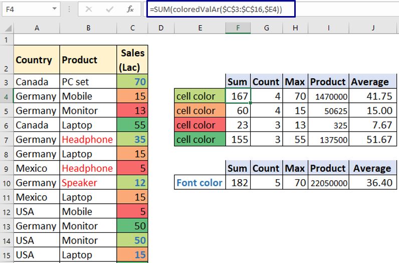
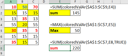
Now you just have to wrap coloredValAr function in functions like Sum, Count, Max, Min, Product,Average ETC. as per your need.
Cell F4 formula =SUM(coloredValAr($C$3:$C$16,$E4)) , cell G4 formula =COUNT(coloredValAr($C$3:$C$16,$E4)) , cell H4 formula =MAX(coloredValAr($C$3:$C$16,$E4)) , cell I4 formula =PRODUCT(coloredValAr($C$3:$C$16,$E4)) , cell J4 formula =AVERAGE(coloredValAr($C$3:$C$16,$E4))
Cell F10 formula =SUM(coloredValAr($C$3:$C$16,$E10,TRUE)) , cell G10 formula =COUNT(coloredValAr($C$3:$C$16,$E10,TRUE)), likewise you can apply formula for Max, Product,Average.
Sum conditionally formatted cell color or font color
Easiest and straightforward way to do this is to create duplicate column of conditionally formatted range which only has color format not conditional formatting.
After this you can use any of the above method to do sum or any other calculations based on color considering duplicate columns with color as reference.
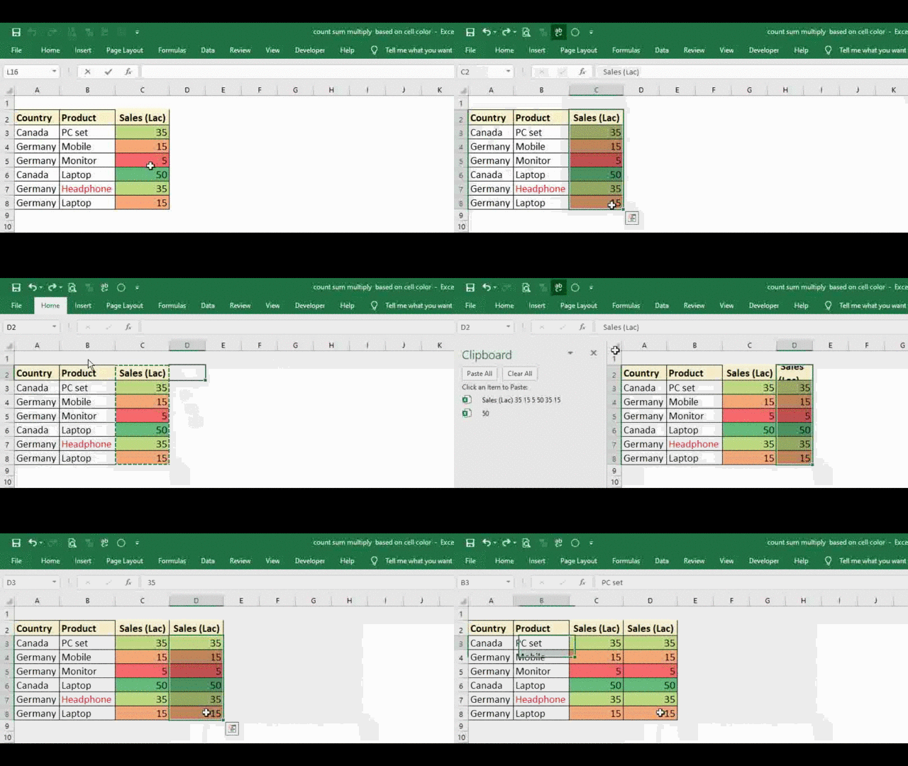
You can also follow the video link to remove conditional formatting and keeping format color trick
Count particular cell color in a range
If you ever encountered a case where you have to count a specific color cells in Excel sheet range then this Excel VBA UDF you can use.
Copy paste below code section in a standard module to make Excel VBA UDF.
Function coloredCellsCount(rng As Range, equalToClrCel As Range) As Long
   Dim cel As Range, cnt As Long, mtClr As Long
   mtClr = equalToClrCel.Interior.Color
   For Each cel In rng
      If cel.Interior.Color = mtClr Then
        cnt = cnt + 1
      End If
   Next cel
   coloredCellsCount = cnt
End Function
=coloredCellsCount(range,coloredCellRng)
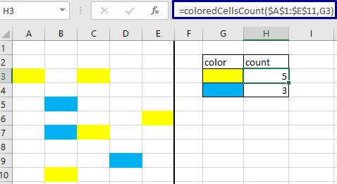
cell H3 formula =coloredCellsCount($A$1:$E$11,G3)
1st input is range in which colored cells are present
2nd input is which cell which contains match color.
