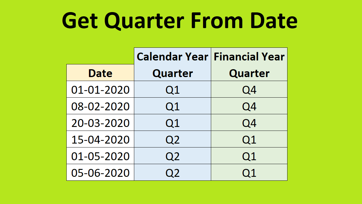
Many times you may need to summarize the data from date wise to quarterly basis. For this, you need to calculate the quarter from the date value.
In Excel, there is no inbuilt function to get quarter from a date.
In this tutorial, you will learn 5 ways to get quarter from a date in Excel.
Quarter from date using Ceiling function
Calendar year quarter
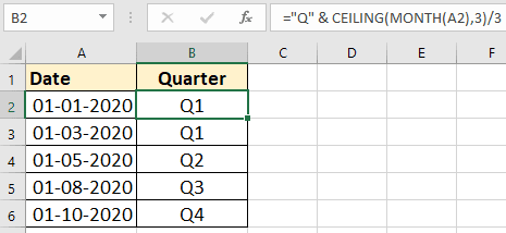
In calendar year 1st quarter begins with Jan month.
In the below image you can see cell B2 formula is
=”Q” & CEILING(MONTH(A2),3)/3 this formula outputs Q1
Formula working:-
MONTH(A2) will give 1. CEILING(1,3) will output 3.
Thus 3/3 will give 1 and this is concatenated with the letter “Q”.
Similarly, if the month is 5th then CEILING(5,3) will output 6 and 6/3 is 2 (quarter 2).
Watch the video related to Ceiling function in Excel
Financial Year Quarter
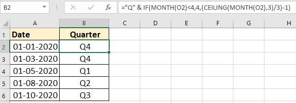
In financial year 1st quarter begins with Apr month.
In the below image you can see cell B2 formula
=”Q” & IF(MONTH(A2)<4,4,(CEILING(MONTH(A2),3)/3)-1)
Note:- If you want only quarter number then don’t concatenate the letter “Q”.
Get quarter using Choose function
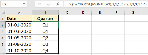
You also use Choose function to get quarter from a Date.
In the below image cell B2 formula for calendar year quarter is
=”Q”& CHOOSE(MONTH(A2),1,1,1,2,2,2,3,3,3,4,4,4)
For financial year quarter use the below formula
=”Q”& CHOOSE(MONTH(A2),4,4,4,1,1,1,2,2,2,3,3,3)
The below image shows the working of the Choose formula for the financial year quarter.
If the month is 1 then 1st value from the series is 4 hence 4 will be output.
If the month is 12 then the 12th value from the series is 3 hence 3 will be output.
Watch the video related to Choose function in Excel

Using approximate Vlookup to get quarter
To get quarter from date using Vlookup you need to first set a reference table.
In the below image reference table is on the right side.
Here I have not used the “Q” letter prefix.
Cell B2 formula for calendar year quarter
=VLOOKUP(MONTH(A2),$F$1:$G$6,2,TRUE)
Cell C2 formula for financial year quarter
=VLOOKUP(MONTH(A2),$F$1:$H$6,3,TRUE)

If you don’t want to refer a table then you can embed the table as an array in Vlookup formula like below.
So, cell B2 formula for calendar year quarter becomes
=VLOOKUP(MONTH(A2),{1,1;4,2;7,3;10,4;12,4},2,TRUE)
Custom function (VBA UDF) to get quarter from date
Quarter function syntax
Quarter(date,RootMonthNo)
The quarter function takes two parameters.
Date is date
RootMonthNo is 1st month number of the 1st quarter (1st quarter starting month).
Example:- In the calendar year, 1st month number of the 1st quarter is 1 (Jan).
In Financial year 1st month number of 1st quarter is 4 (Apr).
Cell B2 formula to get calendar year quarter
=Quarter(A2,1)
Cell C2 formula to get financial year quarter
=Quarter(A2,4)
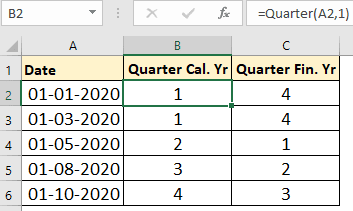
Below is the code for the Quarter custom function (VBA UDF). You need to paste this code in the standard module.
Learn more about creating Excel VBA User Defined Function
Function Quarter(dt As Variant, rootMnthNo As Variant) As Byte
'' dt is date
''rootMnthNo is 1st month number of 1st qrtr
Dim mnth As Byte, nxtMnth As Byte
Dim cntr As Byte
mnth = Month(dt)
nxtMnth = rootMnthNo
For cntr = 1 To 12
     Quarter = Application.WorksheetFunction.Ceiling(cntr, 3) / 3
     If mnth = nxtMnth Then Exit Function
     If nxtMnth = 12 Then
        nxtMnth = 1
     Else
        nxtMnth = nxtMnth + 1
     End If
Next cntr
End Function
Using Pivot table group by quarter feature
If you want to consolidate data from date wise to quarter wise then you can use group by feature of the pivot table.
First, make a pivot table.
Drag date field in Row section.
Select any cell of the Date pivot field and right-mouse click. Click on the Group option.
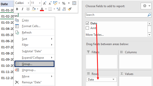
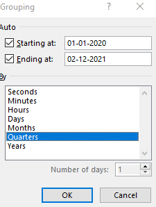
In grouping options, select Quarters then click on the OK button.
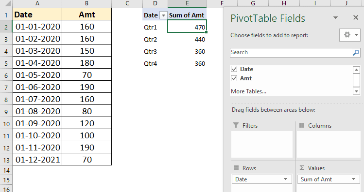
Select field to be summarized in Values section of pivot field.
Watch video Excel Pivot Trick – Group dates into month, year ,quarter
You may also like to explore the below topics
4 Ways to do Running Total in Excel | Cumulative Total in Excel
