In this Excel-related article, you will learn how to get first, second, and Nth visible cell values on a filtered range.

Two methods are shown

• Using helper column and Match Index function
• Using VBA User-Defined function

https://learnyouandme.com/wp-content/uploads/2022/06/Get-first-2nd-Nth-visible-cell-value-after-filter-in-Excel-3.mp4

Nth visible cell value in filtered range using formula

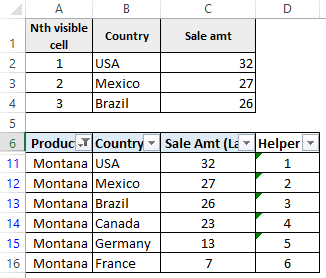
In the below image after applying filter in a table (starting with row 6) 

• 1st three visible countries and their respective sales amt. should be updated in the table above it.

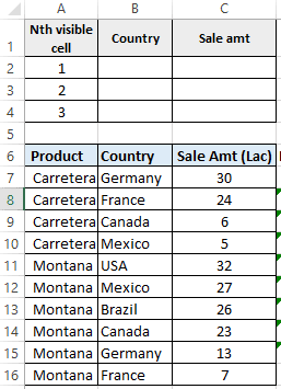
Follow the below steps

• Build a helper column like the below.
• This helper column has the Subtotal formula for running CountA function.

Cell D7 formula =SUBTOTAL(3,$C$7:C7)

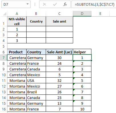
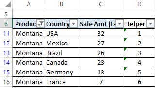
What this formula does is that it dynamically maintains the serial number even after applying the filter.

In the below image you can serial number auto changes after applying the filter.

This helper formula column is the heart of the solution.

Now you just need a combination of the Match and Index function.

Cell B2 formula =INDEX($B$7:$B$16,MATCH($A2,$D$7:$D$16,0),1)

Cell C2 formula =INDEX($C$7:$C$16,MATCH($A2,$D$7:$D$16,0),1)

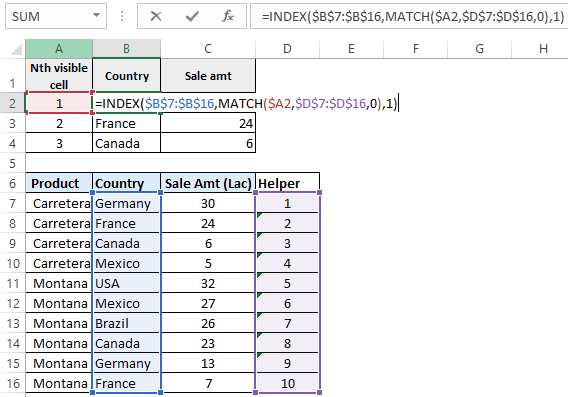
In the below image Montana is filtered and 1st three visible cell values got updated in the upper table.

Below is the formula evaluation for 1st visible cell value in the Country column

In Match function 1st input A2 represents Nth visible cell, you can also put hard value instead of a cell reference.

=INDEX($B$7:$B$16,MATCH($A2,$D$7:$D$16,0),1) then

=INDEX($B$7:$B$16,MATCH(1,$D$7:$D$16,0),1) then

=INDEX($B$7:$B$16,5,1) outputs USA since Index function returns Range as output.

Download file – Get first, 2nd, Nth visible cell value after filter in Excel

First, 2nd, Nth visible cell value of filtered range using VBA UDF function

Instead of building a helper column to get the Nth visible cell value, you can build UDF (User Defined Function) for this.

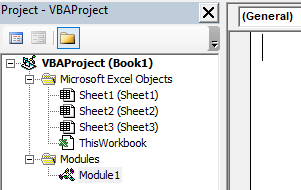
• To make UDF press ALT+F11 to open VBA IDE
• In VBA IDE click on the Insert tab then click Module to create a standard module
• Copy-paste the below code section in that newly created module.

The function name is Nth_VisibleCell and takes two inputs.

1st input is the range and 2nd input is which Nth visible cell value you want.

Function Nth_VisibleCell(rng As Range, NthNo As Integer) As Range
  Dim cel As Range, i As Integer
 If NthNo > rng.Rows.Count Then Exit Function
  For Each cel In rng
    If cel.EntireRow.Hidden = False Then
     i = i + 1
     If i = NthNo Then
        Set Nth_VisibleCell = cel
        Exit Function
     End If
    End If
  Next cel
End Function

Note:- You must insert the above code section in the Standard module only else you can not use UDF in the cell.

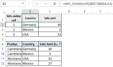
Cell B2 formula =Nth_VisibleCell($B$7:$B$16,A2)

Cell C2 formula =Nth_VisibleCell($C$7:$C$16,A2)

Go to this link to learn more about UDF functions in Excel

You may also like to read Get first/last non-blank cell value in a range | Coalesce function in Excel

Here is another interesting video similar to this topic but a different method is used.

Auto change table heading after filter | Get value from the first visible cell in the filtered range

Download file – auto change table heading after filter in Excel

https://youtu.be/1PXDLzWzZ7o