Say bye to manually giving grades to marks in Excel based on mark range. 

Even if you have used nested and complicated IF function for giving a grade, here I will share a very simple and easy way to give grading to marks in Excel without using the IF function.

Using this technique you can expand your grades without complicating the formula.

Marks grade formula in Excel using approximate Vlookup

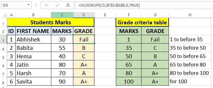
Here you can see total 5  grades (A+, A, B, C, Fail) used to give grading based on marks range.

In Cell D3 approximate Vlookup formula is used to give grading based on marks.

Cell D3 formula : =VLOOKUP(C3,$F$3:$G$8,2,TRUE)

Note: In approximate Vlookup last parameter (4th input) must be TRUE or 1.

Before applying the approximate Vlookup formula first build a reference table (Grade criteria table) .

This reference table must have

1. Marks and Grade column. The marks column must be first.
2. Mark must be in ascending order (small to large).
3. Marks must be as per your grade criteria.

Example: If 1 to before 35 grade is a “Fail” then 1 must be in the 1st row and 35 in the 2nd row.

In the above image, I have written an explanation in the “H” column to understand how the approximate Vlookup formula reads the reference table and populates the grade output.

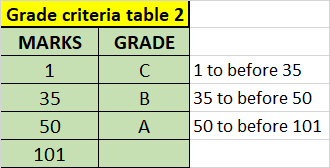
Look at the below image for what will be the reference table, if the grading criteria is changed.

Advantages of approximate Vlookup for grading marks

1. Formula building is fast, simple, and clean.
2. You can easily change the reference table if your criteria rule is changed. 
3. You can easily have N number (5 or more) of grades without any complexity.

Just imagine what if will If function there are more the 3 types of grades. It will be very complex nested if function.

Grading to marks using IF function in Excel

Yes, you can use IF function for giving grades.

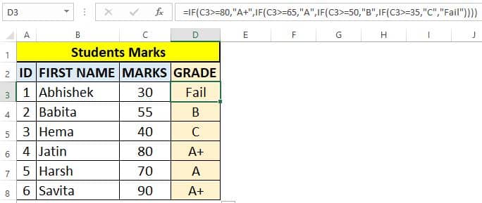
In the below image, you can see a nested IF function for giving grades.

Cell D3 formula :  =IF(C3>=80,”A+”,IF(C3>=65,”A”,IF(C3>=50,”B”,IF(C3>=35,”C”,”Fail”))))

You can clearly see how much careful multiple IF nesting is required for just 5 types of grading.

Just imagine if grading is 5 or more types, how much difficult and complex will be nested IF formula?

So, we can clearly conclude approximate Vlookup formula is the winner.  

Download file – Grade formula in Excel