Do case sensitive Vlookup (lookup) in Excel

Issue with Vlookup and Index Match

Vlookup and Index Match functions are great for lookuping up a value from a table or range.

But, one of the issue with these functions is that they are not case sensitve. These functions treat text “ABC” and “abc” as equal text.

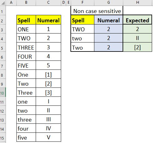
In the the below image left table is lookup table or table array in the right table Vlookup is applied in Light blue range.

You can see in all cases Vlookup is outputting 2 but we expect output as per green range.

So in this post I will show you 3 ways to make case sensitive lookup or Vlookup in Excel.

non case sensitive vlookup

Case sensitive lookup using array formula (Index+Match+Exact array formula)

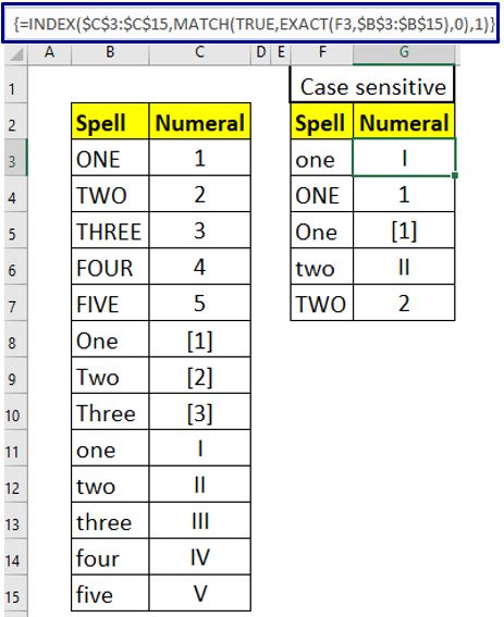
Cell G3 formula =INDEX($C$3:$C$15,MATCH(TRUE,EXACT(F3,$B$3:$B$15),0),1)

In the below image you can see curly brackets around formula which indicates it is an array formula.

So after writing formula press CTRL+SHIFT+ENTER insted of ENTER key to make it array formula.

case sensitive vlookup in excel using array formula

Working of array formula

=INDEX($C$3:$C$15,MATCH(TRUE, EXACT(F3,$B$3:$B$15) ,0),1)

If you look at the above formula then everything is similar to lookup using Index Match function.

In Match function Exact function (yellow section) is outputting an array of boolean values (true or false) which represents whether cell F3 value (“one”) is matched with values in range B3 to B15 spelling-wise and case-wise both.

Select Exact function (yellow part) press F9 function key to see formula evaluation, you will see an array like below one

=INDEX($C$3:$C$15,MATCH(TRUE, {FALSE;FALSE;FALSE;FALSE;FALSE;FALSE;FALSE;FALSE;TRUE;FALSE;FALSE;FALSE;FALSE} ,0),1)

Above you can see TRUE is there at cell B11 (“one”) position which is exactly equal (spell and case wise) to cell F3 value.

Now you just have to find TRUE position in an array using Match function.

=INDEX($C$3:$C$15,9,1) in cell G3 Match is outputting 9 which means cell F3 value (“one”) is at 9th postion in range B3 to B5.

Now you just have to apply Index to get correct Numeral sign.

Using helper column and helper UDF

Main idea behind second method is that to convert lookup values into their respective codes.

=CODE(“A”) will output 65 and =CODE(“a”) will output 97. As you can see for same spelling or letter code is different for uppercase and lowercase.

if you write =CODE(“Aa”) then this will output 65, code of 1st letter only but we want code of both. So for this one UDF (User Defined Function) is needed.

Function f_stringToCode(str As Variant) As String
 Dim nStr As String, i As Integer
 Dim sLen As Integer
 sLen = Len(str)
 nStr = ""
 For i = 1 To sLen
    nStr = nStr & Asc(Mid(str, i, 1))
 Next i
 f_stringToCode = nStr
End Function

As you can see above UDF is f_stringToCode. This UDF will output code of string.

=f_stringToCode(“Aa”) will output 6597 which is concatenate of code of “A” = 65 and “a” = 97.

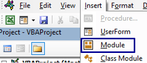
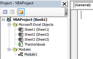
To create above UDF press ALT+F11 to open VBA IDE. In VBA IDE go to Insert tab and click on Module to create new standard module. Now copy past above code section in that module.

Make sure to save as your workbook either in .xlsb (binary) or .xlsm (macro) format.

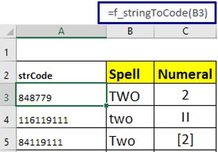
Creating Standard module in Excel VBA IDE
standard module in VBA

Now create one new column for string code at left most of lookup table like the below image. Cell A3 formula =f_stringToCode(B3)

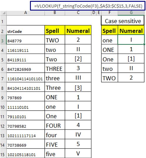
Now this string to code column becomes our lookup column of lookup table.

string to code vba udf

Formula used in cell G3 =VLOOKUP(f_stringToCode(F3),$A$3:$C$15,3,FALSE)

f_stringToCode(F3) will output string code which will be used as lookup value.

After f_stringToCode(F3) evaluation Vlookup formula looks like below

=VLOOKUP(111110101,$A$3:$C$15,3,FALSE)

case sensitive vlookup in excel using helper column and helper UDF

Case sensitive lookup using direct UDF

Copy paste the below code in the Standard Module of VBA IDE. Please refer above method 2 for creating stanadard module in Excel.

As you can see UDF function name is f_caseLookup and requires 3 inputs.

1st input is lookup value , 2nd is lookup range / column and 3rd is output range /column.

Function f_caseLookup _
(lVal As Variant, lookupRng As Range, outRng As Range) As Variant
    Dim lookupRngAr As Variant, ttlVals As Long
    Dim val As Variant, Idx As Long
    lookupRngAr = lookupRng.Value
    Idx = 1
    For Each val In lookupRngAr
        If val = lVal Then
            Exit For
        End If
        Idx = Idx + 1
    Next val
    If outRng.Columns.Count = 1 Then
        'if vertical lookup
        f_caseLookup = outRng.Cells(Idx, 1)
    Else
        'if horizontal lookup
        f_caseLookup = outRng.Cells(1, Idx)
    End If
End Function

Cell E3 formula =f_caselookup(D3,$A$2:$A$14,$B$2:$B$14).

D3 is lookup value

$A$2:$A$14 is lookup column of table

$B$2:$B$14 is output column, whose value we want in lookup output.

case sensitive excel lookup VBA UDF

Issue with Vlookup and Index Match

Case sensitive lookup using array formula (Index+Match+Exact array formula)

Working of array formula

Using helper column and helper UDF

Case sensitive lookup using direct UDF

Leave a Comment Cancel reply