Excel VBA UDF

By default any lookup function like Vlookup, Hlookup, Index Match return only the first matched value. But there are scenarios where you may want to return all matched duplicate values like the below image.

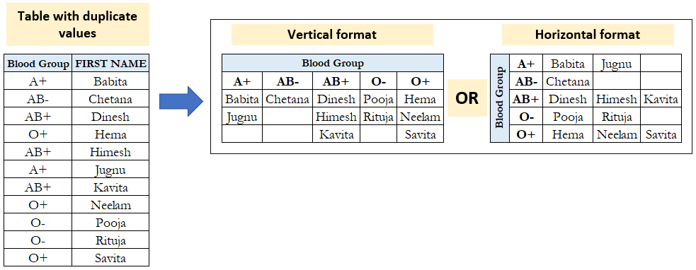
In the above image you can see leftmost table has Blood Group column with duplicate values. We want duplicate value lookup or output all matched Names of a blood group as in right tables.

Vlookup to return all matched values using helper column

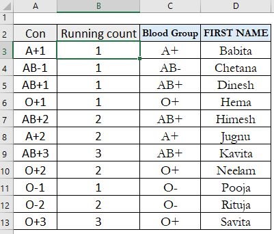
This method is very easy and straightforward. The main idea behind this method is to create one unique column with concatenate lookup value and running count of lookup value.

Cell B3 formula =COUNTIF($C$3:C3,C3) will give running count of Blood group values.

Cell A3 formula =CONCATENATE(C3,B3)

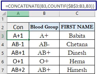
Instead of creating two helper columns, you can merge running count formula in concatenate formula of cell A3 itself like below. 

Cell A3 formula =CONCATENATE(B3,COUNTIF($B$3:B3,B3))

After this you can delete Running count column. This concatenate column will be lookup column for Vlookup function.

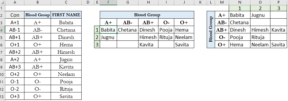
Cell F4 formula for vertical format =IFERROR(VLOOKUP(CONCATENATE(F$3,$E4),$A$2:$C$13,3,FALSE),””)

Iferror function is there for hiding #N/A error, CONCATENATE(F$3,$E4) outputs lookup value (A+1 ).  

Cell N2 formula for vertical  format  =IFERROR(VLOOKUP(CONCATENATE($M2,N$1),$A$2:$C$13,3,FALSE),””)

Vlookup to return all matched values using array formula without helper column

Cell F4 formula =IFERROR(INDIRECT(“C”&SMALL(IF($B$3:$B$13=F$3,ROW($B$3:$B$13),””),$E4)),””)

cell N2 formula =IFERROR(INDIRECT(“C”&SMALL(IF($B$3:$B$13=$M2,ROW($B$3:$B$13)),N$1)),””)

In the image you can see curly brackets at the end which mean it is an array formula.

So press CTRL+SHIFT+ENTER instead of ENTER key to make it array formula.

Woking of array formula

=IFERROR(INDIRECT(“C”&SMALL(IF($B$3:$B$13=F$3,ROW($B$3:$B$13),””),$E4)),””)

Above If section will produce array row numbers in which blood group is matched.

If you select If section (yellow) of cell F4 formula and press F9 then you will see something like below.

{3;””;””;””;””;8;””;””;””;””;””} this basically means matched blood group (A+) is present in 3rd and 8th row of Excel sheet.

SMALL({3;””;””;””;””;8;””;””;””;””;””},$E4) here in E4 to E6 range matched serial is written.

so for 1st serial Small will give 3 and for 2nd 8

INDIRECT(“C”& 3) represents cell C3 and cell C3 value is Babita likewise

INDIRECT(“C”& 8) represents cell C8 and cell C8 value is Jugnu

Entire Indirect function is wrapped in Iferror function to handle not matched values.

Vlookup to return all matched values using VBA UDF (User Defined Function)

Option Explicit
Option Compare Text
Function lookupNthValue(lkVal As Variant, lkRng As Range, _
outRng As Range, mtchInst As Long) As Variant
    If mtchInst = 0 Then
        lookupNthValue = ""
        Exit Function
    End If
    Dim lkRngAr As Variant, i As Long, j As Long
    Dim findedIdx As Long, clmnCnt As Byte
    clmnCnt = lkRng.Columns.Count
    If clmnCnt = 1 Then
      lkRngAr = Application.Transpose(lkRng.Value)
    Else
      lkRngAr = Application.Transpose(Application.Transpose(lkRng.Value))
    End If
       findedIdx = Application.Match(lkVal, lkRngAr, 0)
       j = 1
    If mtchInst > 1 Then
       For i = findedIdx + 1 To UBound(lkRngAr)
          If lkRngAr(i) = lkVal Then
             findedIdx = i
             j = j + 1
          End If
          If j = mtchInst Then Exit For
       Next i
    End If
      If j < mtchInst Then
        lookupNthValue = ""
        Exit Function
      End If
     If clmnCnt = 1 Then
       lookupNthValue = outRng.Cells(findedIdx, 1)
     Else
       lookupNthValue = outRng.Cells(1, findedIdx)
     End If
End Function

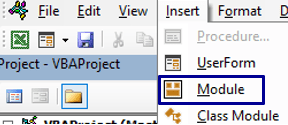
To create above UDF press ALT+F11 to open VBA IDE. In VBA IDE go to Insert tab and click on Module to create new standard module. Now copy paste above code section in that module.

Make sure to save as your workbook either in .xlsb (binary) or .xlsm (macro) format.

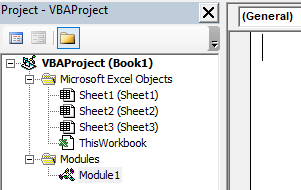
After copy pasting UDF in Module you are ready to use lookupNthValue UDF function in Excel cell.

Cell F4 formula =lookupNthValue(F$3,$B$3:$B$13,$C$3:$C$13,$E4)

lookupNthValue  takes 4 inputs

1st input is lookup value (for cell F4 formula it is A+)

2nd input is lookup range ($B$3:$B$13 represents range in which lookup value is present)

3rd input is output range (since we want First Name hence output is $C$3:$C$13)

4th input is number which means which Nth match you want to output

=lookupNthValue(F$3,$B$3:$B$13,$C$3:$C$13,1) will output 1st match Babita

=lookupNthValue(F$3,$B$3:$B$13,$C$3:$C$13,2) will output 2nd match Jugnu for A+ blood group.

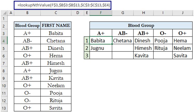
Note:- If match not found and if 4th input is 0 then lookupNthValue function will output blank string.

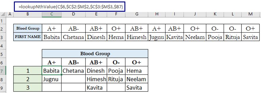
You can use lookupNthValue  UDF for looking up horizontal table also like the below image.

Cell C7 formula =lookupNthValue(C$6,$C$2:$M$2,$C$3:$M$3,$B7)

You may also like to read the below topics

Return multiple Vlookup values in one cell (Text join if) 3 ways

Reverse Vlookup In Excel (Vlookup Right to Left)

Master Vlookup with multiple columns criteria and double Vlookup

You can also watch the below video of  Vlookup to return multiple matched values |Vlookup for multiple matched value (Method 3) in Hindi speech.

https://youtu.be/oR1fOe2p34U