In this Excel tutorial, you will learn how to calculate various types of percentages in Excel.
I have tried to include common types of percentages like percent discount, GST percentage (GST% ,GST amount, reverse GST) or GST formula in Excel , percentage marks, percent contribution from total or percent mix, markup and markdown percentage and gross margin percent calculation in Excel.
Excel formula for percentage discount (discount rate)
To find the percentage discount or discount rate in Excel follow the below steps.
- Find the difference between MRP and Sale Rate
- Divide difference amount by MRP
- Format discount rate values as percentage
Discount Rate= (MRP-Sale Rate)/MRP *100 (without percent sign in the cell)
or Discount Rate= (MRP-Sale Rate)/MRP (with percent sign in a cell formatted as percent)
Cell D10 formula =B10-C10
Cell E10 formula =D10/B10
Alternatively, you can directly calculate percentage discount without helper column like below
In cell D10 you can directly write =(B10-C10)/B10 to find discount rate in Excel.

To show the percentage sign in discount rate follow the below steps
- Select discount rate cells
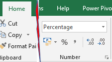
- Go to Home tab the select percentage format from the dropdown.
Alternatively, select range then press CTRL+SHIFT+% shortcut key to bring the number in a percentage format.
Show and remove percentage sign in Excel | Percentage to a number

Calculate price after discount in Excel
You can calculate price after discount using MRP and discount rate in Excel.
Follow the below steps
- Find discount amount (MRP*Discount percent)
- Subtract this discount amount from MRP
Discounted Price = MRP-Discount amount
or Discounted Price = MRP-(MRP*Discount percent)
or Discounted Price = (100%-Discount percent)*MRP
Cell D2 formula =B2-(C2*B2)

If in discount value % sign is not there then use the below formula to get the original price after discount.
Just add percent sign after discount value cell address
Cell D2 formula =B2-(C2%*B2)

Alternatively, you can use the below formula
Cell D2 formula =(100%-C2)*B2
The above calculation concept is like below
If there is a 10% discount then you will pay 90%. So to get the price after discount just multiply the pay percentage 90% by MRP.

How to find the original price before discount ?
Suppose you have discount percentage and rate after discount in Excel sheet, here you want to get the original price before discount or undiscounted price.
In the below image price after discount and discount rate is known, you have get the original price before discount means MRP.
Cell D2 formula is =B2/(100%-C2)
Here is a breakdown or understanding for “Earphone A10”
In Cell D2
- (100%-C2)=(100%-10%) will give 90% ( can be written as 90/100) which is a portion of the original price one needs to pay after the discount.
- B2/(100%-C2) =B2/90%=450/(90/100)
- Rearranging 450/(90/100) will give (450/90)*100. Here (450/90) will give the price of 1% portion.
- When (450/90) multiplied by 100 you will get the price of 100% portion which is the original price before discount.

Note:- If you are not using percentage sign in discount rate then the cell D2 formula will be like below.
=B2/(100-C2)*100

Calculate GST tax amount in Excel
In the below image taxable amount (rate without tax) and GST rate is given.
To calculate GST tax amount you can use the below formula
GST Amount = Taxable Amount*GST Rate%
or
GST Amount = Taxable Amount*(GST Rate/100)
Cell D2 formula =B2*C2% , since there is no percent sign in GST rate
Cell D4 formula for GST Amount =B4*C4, since there is a percent sign in GST rate.
After calculating the GST tax amount you can get the Amount with GST using the below formula
Amount with GST tax = Taxable amount + GST amount
Cell E2 formula for amount with GST tax =B2+D2

Reverse GST calculation formula in Excel (GST reverse charge)
Many struggles to calculate the taxable amount and GST amount when the amount with tax and tax rate (GST rate) is provided in Excel.
Below is the formula for reverse GST calculation (GST reverse charge)
Taxable Amount = Amount with tax / (100+GST rate)*100
GST Amount = Amount with tax / (100+GST rate)* GST rate
Cell D2 formula for taxable amount =B2/(100+C2)*100
Cell E2 formula for GST amount =B2/(100+C2)*C2
Alternatively, you can also get GST amount by subtracting Amount with tax with taxable amount.

If the GST rate has a percent sign then use then instead of only 100 use 100% in the formula.
cell D2 formula =B2/(100%+C2)*100%
cell E2 formula =B2/(100%+C2)*C2
So, in reverse GST calculation, you split the amount with tax into the taxable amount and GST amount.

Excel formula for percentage of total in Excel
Sometimes you may need to calculate the percentage of total value in Excel.
By calculating percentage of total you can know the mix percent or percent contribution of each element.
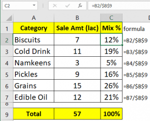
In the below table category and sale amount is given.
To calculate the mix percentage or percentage contribution of each category in total sale value, do the below steps.
- Calculate total sale amount by applying Excel Sum function
In cell B9 total is calculated using formula =SUM(B2:B8)
- Divide individual value with total amount
cell C2 formula =B2/$B$9. Now select cells (C2:C7) then press CTRL+SHIFT+% to show percentage sign (format number as a percentage).
If you do not want to show the percentage sign then the cell C2 formula becomes =B2/$B$9*100, keep cell or range format to “General” or number format.

Percentage of subjects marks Excel formula
Students and teachers require to calculate the percentage of marks in a given subject.
To calculate marks percent just divide marks got by max marks.
Marks percentage = Marks got / Max marks (format cell as a percentage to show percent sign)
or
Marks percentage = Marks got / Max marks * 100 (keep cell format general or number to show numbers without the percent sign)
Cell D2 formula =C2/B2
After applying the formula, select cells then press CTRL+SHIFT+% to apply percentage number format on cell.

Calculate percentage increase or decrease (percent change) in Excel
In the below image quarter wise sale of two years is given.
Step to calculate percentage increase decrease (% Growth) in Excel
- Find the difference between the latest year’s sales and the past year’s sales.
Growth amount = Latest year sale – Past year sale
Cell D3 formula =C3-B3
- Divide Growth amount by past year sale
Percentage growth = Growth amount/ Past year sale (format cells to percentage to show percent sign)
or
Percentage growth = Growth amount/ Past year sale *100 (keep number format general or number – without the percent sign)
Cell E3 formula =D3/B3

To calculate percentage increase and decrease directly, without using the growth amount column use the below formula.
Cell D3 formula =(C3-B3)/B3 (format cell to percentage to show % sign)
If you do not want to show the percentage sign then use the below formula and keep the cell format general or number.
Cell D3 formula =(C3-B3)/B3*100

Calculate markup and markdown percentages in Excel
Markup and markdown percentage
Markup percentage is on each 100 rupees cost, how much amount you want to add.
Markdown percentage is on each 100 rupees value, how much amount you want to subtract.
Calculation steps
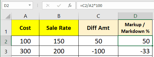
- Find the difference between sale rate and cost
- Divide difference amount by COST amount then multiply it with 100
Cell D2 formula =C2/A2*100
If you want to show a percentage sign then do not multiply it with 100 and change cell format to the percentage by pressing CTRL+SHIFT+%
In the second example markdown is done.

Calculate original price before markdown in Excel
Here you have markdown rate and amount after markdown, you want to find out the price before markdown.
Original price = Price after markdown / (100- markdown rate) *100
Cell C2 formula =(A2/(100-B2))*100
Note:- If markdown rate has percentage sign then use below formula
Cell C2 formula =(A2/(100%-B2))*100%

Calculate price after markup in Excel
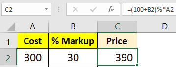
Price after markup = (100+markup rate)%*Cost
or Price after markup = Cost + (Cost/100)* markup rate
Cell C2 formula =(100+B2)%*A2
If markup rate has % sign then C2 formula =(100%+B2)*A2
Intuitive explanation:- Markup rate is on every 100 rupees, how much amount you want to add.
So, in 300, three 100 rupees are there (100+100+100)
For 30% markup rate total value will be add 30 Rs. on each 100 (30+30+30) =90
Price after after markup = 300 + 90 = 390

You can also watch below video in Hindi
Calculate % gross profit , reverse GST, percent markdown & markup in Excel | Reverse charge in GST
You may also like to read
Show and remove percentage sign in Excel | Percentage to a number
Gross margin percentage calculation in Excel
Definition:- Gross margin percentage is on each 100 rupees sale, how much profit is made.
Note:- Gross margin is calculated on each 100 rupees sale not cost.
Follow the below steps to get the Gross margin percentage
- Find Gross profit amount by subtracting Sale with Cost
- Divide Gross profit amount by Sale then multiply it with 100
Gross margin percent = (Gross profit amount/Sale amount) *100
or Gross margin percent = ((Sale amount- Cost amount)/Sale amount) *100
cell D2 formula =C2-B2
cell E2 formula =(D2/C2)*100

How to add 5 percent to a number in Excel?
To add 5 percent to a number or increase any number by X percent, one can use one of the below formulas.
Increase number by X% = (100%+Increment %)*Number
cell C2 formula =(100%+B2)*A2
Use this formula when increment number percent has % sign

If increment number percentage do have % sign then use the below formula
Cell C2 formula
=(100+B2)%*A2

Alternatively, you can use the below formula to add 5 percent to a number
Increase number by X% = (Number*Increment %) + Number
Cell C2 formula =(A2*B2%)+A2
Notice in the below image 5 does not have percent sign.
If 5% is written instead of 5 then formula will be
cell C2 formula =(A2*B2)+A2

You can also watch below video in Hindi
How to calculate percentage in Excel | Percent increase in Excel
https://youtu.be/B9qWlKWwpjs