Sometimes you may need to compare two or more Excel columns to find the matches and differences.
Here I have discussed various scenarios and respective methods to compare values in Excel columns.
Compare two columns in Excel row wise
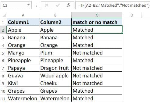
In the below example scenario, you can see two columns are compared for matched values.
Simple If formula is used to find the row wise matched and not matched values between columns.
Cell C2 formula
=IF(A2=B2,”Matched”,”Not matched”)
Compare two columns exact case wise in Excel
In this scenario you not only want to compare 2 columns by value but also by letter case also.
Same If formula can be used but with a little twist.
Cell C2 formula
=IF(EXACT(A2,B2),”Matched”,”Not matched”)
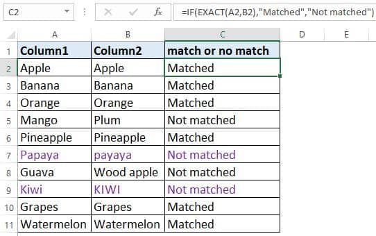
Here you can see in If function Exact function is used to check whether case is also same.
You can see “Papaya” and “Kiwi” example row , here spellings are same but case is different hence formula is outputting “Not matched”.
Compare two columns by highlighting matching rows in Excel
Here is a step by step way to highlight matching rows in Excel using conditional formatting.
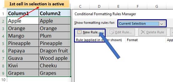
1 – Select range and make sure 1st cell of the selected range is active.
2 – Press the ALT O D keys in series and click on New Rule.
Alternatively, click HOME tab > CONDITIONAL FORMATTING > New Rule
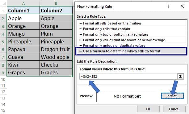
3 – Now click on “Use a formula to determine which cells to format”
4 – Write formula rule =$A2=$B2. Putting $ sign before column is important.
5 – Click on OK button.
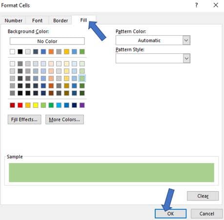
6 – Click on Fill tab. Select highlight color.
7 – Click on OK button and in all upcoming pane click on OK button.
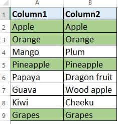
In the below image, you can see matched rows between columns got highlighted.
Same method you can use to highlight not matched rows in Excel
This is how you can visually compare two columns in Excel.
Compare two or more columns of two tables in Excel
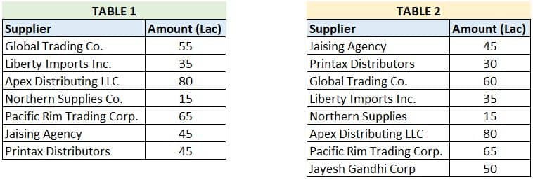
In the below image you can see two tables.
I want to compare both the Supplier name and the respective amount side by side.
In comparison, I want to see missing values, matched values, and not matched values for a given record in the two tables.
These two tables may present in different sheet or different workbooks, it doesn’t matter.
For simplicity in both tables rows are less and the column count is limited to 2 columns.
But using this clean, simple approach you can compare many columns with many number of rows.
Also, you can compare more than tow tables using this approach.
Below is expected output of side by side column comparison.

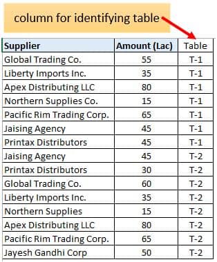
1 – First merge two table one below other to make a big table.
Here you need identify each table records by their table source. In the below image column named “Table” created for this purpose.
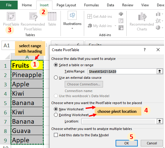
2 – Now select this merged range with heading and create Pivot Table. Follow the below steps.
- Select range then go to the Insert tab and click on Pivot table option.
- Select whether you want to create Pivot in existing or new worksheet.
- Click OK button.
Note:- In the below image table is different. Image only represent steps to follow for making Pivot table in Excel.
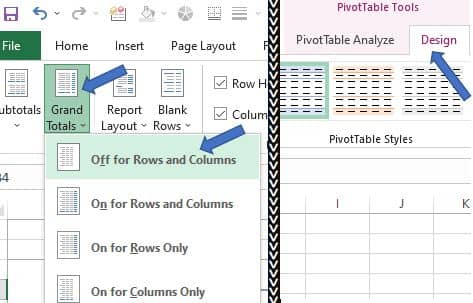
3 – Click on any cell of the pivot table region to bring “PivotTable Tools” tab.
4 – In PivotTable Tools click on Design. Then from Grand Totals drop down list click on “Off for Rows and Columns” option.
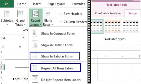
5 – In Report Layout click on Show in Tabular Form and Repeat All Item Labels on by one.
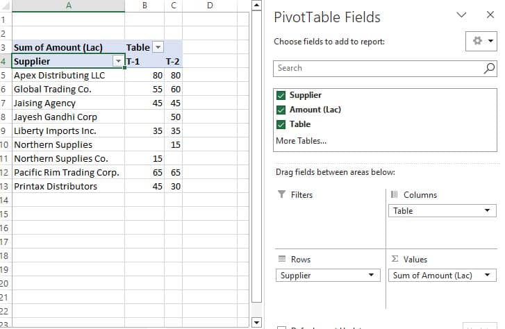
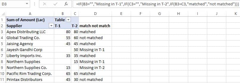
6 – Arrange columns in their respective area as per the below image. Supplier is in the Rows area, table is in Columns, and Amount in the Values area.
As you can see we brought columns of two table (two list) side by side for comparison purposes.
Additionally, you can add a formula column at the end to compare columns for missing, matched and not matched values.
Cell D3 formula
=IF(B3=””,”Missing in T-1″,IF(C3=””,”Missing in T-2″,IF(B3=C3,”matched”,”not matched”)))
Note: Since suppliers will auto get sorted in ascending order you can also see whether mismatch is due to typo error or not. See 8th and 9th row of “Northern Supplies”.
I think using the Pivot table technique is one the best way to compare multiple columns in Excel to find matches and differences.
The below video shows different examples but has the same approach of column comparison in Excel.
https://youtu.be/uV7o4CG6j7A
Download file – compare two columns in excel