In this Excel tutorial, you will learn how to highlight alternate rows in Excel to make the data table more visually pleasing.
Highlighting method discussed here have the below features
- Fast and easy method
- You can quickly change the colour (font and cell) of the alternate rows as your requirement
- Highlighting will auto expand when new data or records are added to the table
Highlighting alternate rows in Excel
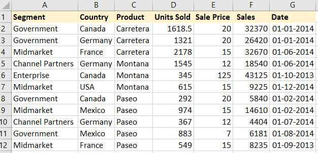
In the below image you can see data table in which highlight alternate rows to be done.

To highlight alternate rows do the below things
- First, select the data range with heading
- Press CTRL+T then Tick on “My table has headers” then click on OK button. Alternatively, you can go to the Insert tab then click on the Table option.
- This will convert the normal Excel table range to an official Excel table also called list object.

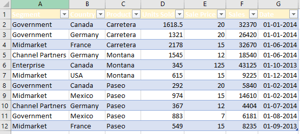
After converting into an official Excel table or list object, the table will look like the below image.
You can see alternate rows got highlighted with light blue colour.
The heading font colour is white but you can simply change it by selecting heading range and changing font colour from Home tab.
When you add a new record (row) or column then highlighting will auto expand to a newly created row or column.

Customising row highlight colour
To customize or change row highlight colour follow the below steps
- Select any cell of the table
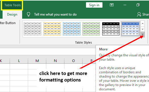
- After selecting a table cell a new Design tab will appear, where you can select different available table styles

In the below image you can see alternate rows got highlighted with new colour after changing table style.

Suggested readings
How to automatically insert serial numbers after filter in Excel?
How to make Microsoft Excel Add in?
How To Convert Number To Hindi Words in Excel?
Suggested Video
Highlight active cell automatically without erasing past cell colour in Excel (Method-2)
https://youtu.be/xssQo3HdrhA