Vlookup with multiple columns criteria
There are many scenarios in Excel where we need to lookup multiple values of different columns at the same time to come across an output. Below image is a perfect example of multiple criteria Vlookup.
In the right table of the below image we need to get amount with matching Name and Area.
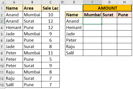
One can solve multiple criteria Vlookup problem using two approaches.
- Using concatenated helper column
- Using Choose formula
Using concatenated helper column for multiple criteria Vlookup
Since we need to get sale amount using Vlookup (typical Vlookup looks up from left to right) hence our helper column with concatenate formula must be present at left side of Sale Lac column which means before C column as per the above image.
So, create one blank column before “C” column like the below image. Write concatenate function concatenating Name and Area values.
=CONCATENATE(A2,B2)
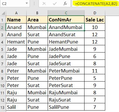
This concatenate function will produce unique combination of values. Unique values combination column is the main idea behind this approach.
One may find scenarios where there may be more than two column values need to be concatenated but approach is same.
One may put separator like dash (-), underscore (_) ETC. between values for better readability and this is optional.
Since our lookup column (helper column) is combination of Name and Area hence lookup value of Vlookup formula must have Name and Area combination in same order.
Formula used =CONCATENATE($F3,G$2)
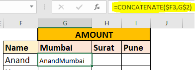
Use concatenated lookup value in Vlookup formula.
Formula used as per the below image
=VLOOKUP(CONCATENATE($F3,G$2),$C$2:$D$13,2,FALSE)
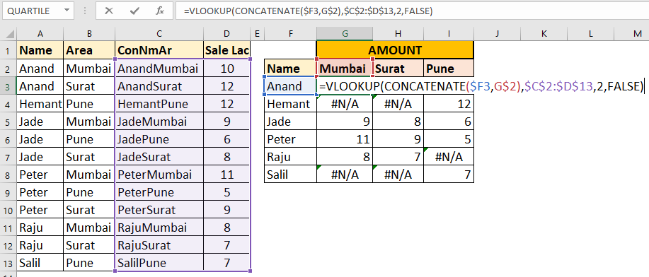
Now to remove #N/A just wrap entire Vlookup formula inside IFERROR function like below
=IFERROR(VLOOKUP(CONCATENATE($F3,G$2),$C$2:$D$13,2,FALSE),0)
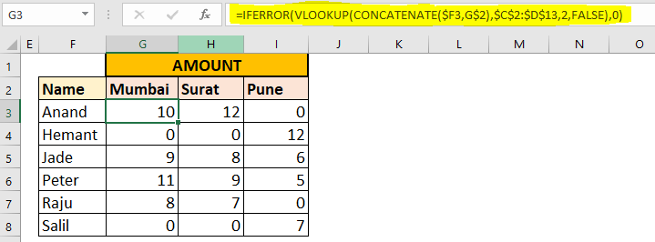
So this is how multiple criteria Vlookup is performed using concatenated helper column.
Advantages of concatenated helper column method
Very clean and simple method.
Can be easily used for doing Vlookup of more than two criterias or columns match.
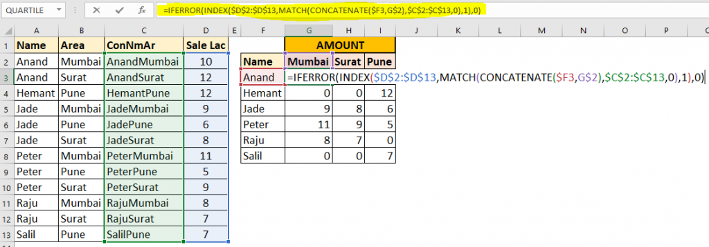
Note:- One can also use Index Match instead of Vlookup in the right table. Index Match will give you flexibility of building helper column at any side (either left or right side) of the Sale amt column.
Formula will look like something below as per example image
=IFERROR(INDEX($D$2:$D$13,MATCH(CONCATENATE($F3,G$2),$C$2:$C$13,0),1),0)
Using Choose function for multiple criteria Vlookup
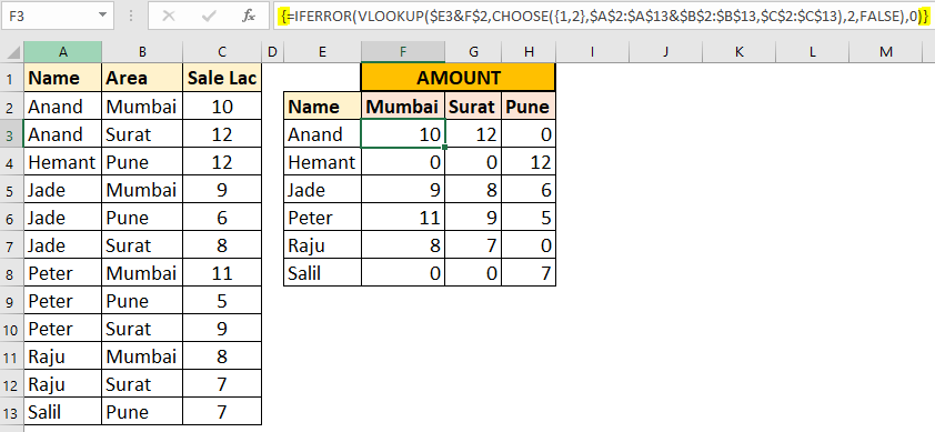
Formula used =IFERROR(VLOOKUP($E3&F$2,CHOOSE({1,2},$A$2:$A$13&$B$2:$B$13,$C$2:$C$13),2,FALSE),0)
If you carefully look at the formula bar in the below image, curly brackets “{}” are there at both end which means it is an array formula.
So instead of pressing ENTER key, press CTRL+SHIFT+ENTER after writing formula to make it an array one.
Now let’s understand working of Choose function for multiple criteria Vlookup.
IFERROR function is fairly simple and clearly shows what it does.
Now carefully look at the below Vlookup formula.
1st yellow section concatenates Name and area, all looks very similar to typical Vlookup function except green part which represents table array of Vlookup.
VLOOKUP($E3&F$2, CHOOSE({1,2},$A$2:$A$13&$B$2:$B$13,$C$2:$C$13) ,2,FALSE)
So somehow this green part is internally getting converted into array or a range having two columns, 1st column is concatenated Name and area and 2nd Sale amt.
Let’s break down this green part CHOOSE({1,2},$A$2:$A$13&$B$2:$B$13,$C$2:$C$13)
$A$2:$A$13 & $B$2:$B$13 internally outputs a concatenated column of Name and Area.
Write =$A$2:$A$13 & $B$2:$B$13 in any cell and press CTRL+SHIFT+ENTER to make it array formula. Now press F2 then F9 you will get output something like below.
{“AnandMumbai”;”AnandSurat”;”HemantPune”;”JadeMumbai”;”JadePune”;”JadeSurat”;”PeterMumbai”;”PeterPune”;”PeterSurat”;”RajuMumbai”;”RajuSurat”;”SalilPune”}
The above array represents lookup column. Now we need to add Sale column.
For adding second column Choose formula is needed.
CHOOSE({1,2}, $A$2:$A$13&$B$2:$B$13 ,$C$2:$C$13) in this $C$2:$C$13 is sale column and {1,2} just simply means output combination of 1st range red one and 2nd range blue one.
Learn right to left Vlookup using Choose function
If you select green part of Vlookup then press F9 then you will get something like below
=IFERROR(VLOOKUP($E3&F$2,{“AnandMumbai”,10;”AnandSurat”,12;”HemantPune”,12;”JadeMumbai”,9;”JadePune”,6;”JadeSurat”,8;”PeterMumbai”,11;”PeterPune”,5;
“PeterSurat”,9;”RajuMumbai”,8;”RajuSurat”,7;”SalilPune”,7},2,FALSE),0)
This output is basically a hardcoded table array instead of range and this all happening behind the scene.
Learn more about embedding table or array values in Vlookup formula
Double Vlookup or Nested Vlookup in Excel
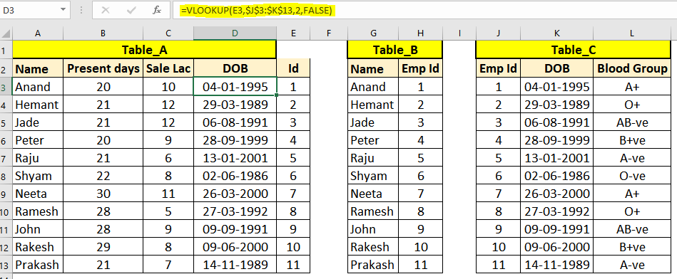
In the Table_A I want DOB (data of birth). This DOB data is present in Table_C. But in Table_A and Table_C there is no common column for making Vlookup.
So how to bring DOB in Table_A?
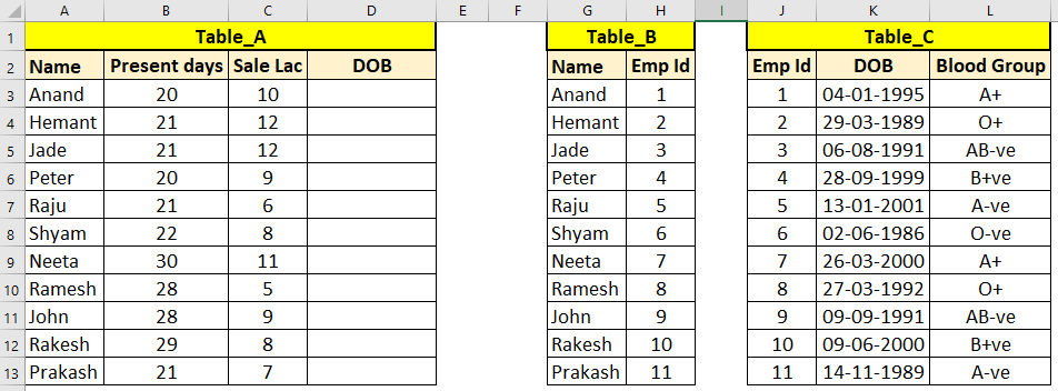
If you see Table_B which provides link (relation) between Name and Emp Id. Now because to this Table_B we can bring DOB in Table_A using 2 approaches.
1st approach – Creating Id column (helper column) in Table A then making Vlookup using Id to Table_C like below image.
For Id output =VLOOKUP(A3,$G$3:$H$13,2,FALSE) formula is used in cell E3.
For DOB output =VLOOKUP(E3,$J$3:$K$13,2,FALSE) formula is used in cell D3.
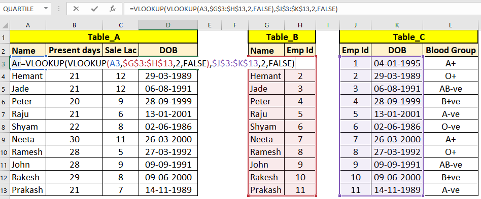
2nd approach- This involves double Vlookup or nested Vlookup in single formula and there is no need to build helper column for this approach.
Cell D3 double Vlookup or nested Vlookup formula
=VLOOKUP(VLOOKUP(A3,$G$3:$H$13,2,FALSE),$J$3:$K$13,2,FALSE)
In the above formula highlighted section (inner Vlookup) will output ID and this ID is used as lookup value for outer Vlookup.
Beginners may not able to comprehend or build mental map of this nested Vlookup formula to make it complex formula.
Below I am giving you a simple strategy to build complex formula.
As you can see Anand Emp Id is 1 , so you can simply put 1 as hard value to output DOB by looking up Table_C
=VLOOKUP(1,$J$3:$K$13,2,FALSE)

Now the second challenge is to how to auto calculate this Id value in the above Vlookup.
For this you just need to Vlookup Name using Table_B as table_array or Vlookup Table.
Make this formula in any blank cell
=VLOOKUP(A3,$G$3:$H$13,2,FALSE)

Now you just need to replace 1 as hard Id value in 1st Vlookup with 2nd Vlookup formula excluding = sign like below. Delete 2nd Vlookup from cell after replacement.

It’s done you have just made double Vlookup or nested Vlookup not requiring helper column.